43 value data labels excel
How to: Display and Format Data Labels - DevExpress To display value labels, set the DataLabelBase.ShowValue property of the DataLabelOptions object to true. Series name. Series labels identify data series to which the data points in the chart belong. Most series include multiple data points, so the same name will be repeated for all data points in the series, which is probably overkill. Pie Chart in Excel - Inserting, Formatting, Filters, Data Labels The chart would consider the absolute ( positive ) value for any negative value in the data ; The total of percentages of the data point in the pie chart would be 100% in all cases. Consequently, we can add Data Labels on the pie chart to show the numerical values of the data points. We can use Pie Charts to represent:
How to add data labels in excel to graph or chart (Step-by-Step) How to use cell values as data labels in excel 1. To display extra data for a data series or data label, right-click it and select Format Data Labels. 2. Select the Values From Cells checked under Label Contains under Label Options. 3.

Value data labels excel
VALUE Function - Formula, Examples, How to Use VALUE in Excel The VALUE Function [1] is categorized under Excel Text functions. It will convert a text string that represents a number into a number. Thus, the function will convert text that appears in a recognized format (a number, date, or time format) into a numeric value. In financial analysis, the VALUE function is not used much, as Excel automatically ... Custom Chart Data Labels In Excel With Formulas - How To Excel At Excel Follow the steps below to create the custom data labels. Select the chart label you want to change. In the formula-bar hit = (equals), select the cell reference containing your chart label's data. In this case, the first label is in cell E2. Finally, repeat for all your chart laebls. How to format axis labels individually in Excel - SpreadsheetWeb The semicolon marks that you passed the next section. If you end with a semicolon, Excel thinks that there won't be a number format for the last section. Mark a single value [Cyan] [=60];General Set different colors for number ranges Since you have three sections for the conditions, you can set up to three colors.
Value data labels excel. excel - Formatting Data Labels on a Chart - Stack Overflow sub charttest () activesheet.chartobjects ("chart 6").activate z = 1 with activechart if .charttype = xlline then i = .seriescollection (1).points.count activechart.fullseriescollection (1).datalabels.select for pts = 1 to i activechart.fullseriescollection (1).points (pts).hasdatalabel = true ' make sure all points are visible data … 13 Essential Excel Functions for Data Entry - How-To Geek Entering data in your spreadsheet is the basic principle behind using Excel. From adding the current date and time to looking up values to changing the letter case of your text, some functions can help you tremendously with data entry. Table of Contents Enter the Current Date and Time: TODAY and NOW How to Add Labels to Scatterplot Points in Excel - Statology Step 3: Add Labels to Points Next, click anywhere on the chart until a green plus (+) sign appears in the top right corner. Then click Data Labels, then click More Options… In the Format Data Labels window that appears on the right of the screen, uncheck the box next to Y Value and check the box next to Value From Cells. How to mail merge and print labels from Excel - Ablebits.com Select document type. The Mail Merge pane will open in the right part of the screen. In the first step of the wizard, you select Labels and click Next: Starting document near the bottom. (Or you can go to the Mailings tab > Start Mail Merge group and click Start Mail Merge > Labels .) Choose the starting document.
How to Print Labels from Excel - Lifewire Select Mailings > Write & Insert Fields > Update Labels . Once you have the Excel spreadsheet and the Word document set up, you can merge the information and print your labels. Click Finish & Merge in the Finish group on the Mailings tab. Click Edit Individual Documents to preview how your printed labels will appear. Select All > OK . How to Create and Customize a Waterfall Chart in Microsoft Excel Go to the Insert tab and the Charts section of the ribbon. Click the Waterfall drop-down arrow and pick "Waterfall" as the chart type. The waterfall chart will pop into your spreadsheet. Now, you might notice that the starting and ending totals don't match with the numbers on the vertical axis and aren't colored as Total per the legend. How to Show Percentages in Stacked Column Chart in Excel? By default, the data labels are shown in the form of chart data Value (Image 1). But very often user needs to plot charts with actual data and show percentages/custom values on the chart instead of default data. For that we have an option "Value From Cells" in chart "Format Data Label" (Image 2) to select a custom range. Image 1 Image 2 Label line chart series - Get Digital Help The data labels now show both numerical values and the last text value. To hide the numerical values simply double press with left mouse button on on the data labels to open the task pane. Deselect check box "Value". All numerical values are now deleted from the data labels, only the last data point has a data label, see image below.
Data label in the graph not showing percentage option. only value ... Normally when you put a data label onto a graph, it gives you the option to insert values as numbers or percentages. In the current graph, which I am developing, the percentage option not showing. Enclosed is the screenshot. Can anyone help me to bring the percentage option as well in this graph data label? Thanks & Regards, Dipil Labels: Excel Excel - "Label Contains: Value from Selected Cells" - two - Microsoft ... Excel - "Label Contains: Value from Selected Cells" - two charts, same data, different label outcomes I have two charts (Scatter plot and Line /w markers) both mapped with the exact same data. How to: Display and Format Data Labels - DevExpress To display value labels, set the DataLabelBase.ShowValue property of the DataLabelOptions object to true. Series name. Series labels identify data series to which the data points in the chart belong. Most series include multiple data points, so the same name will be repeated for all data points in the series, which is probably overkill. How to Edit Pie Chart in Excel (All Possible Modifications) As a result, there will be a new ribbon named Format Data Labels at the right side of your Excel file. Now, go to the Label Options menu >> Label Options group >> put a tick mark on the Percentage option. As a result, there will be percentage values too at the data labels. The result sheet would look like this. 👇 9.
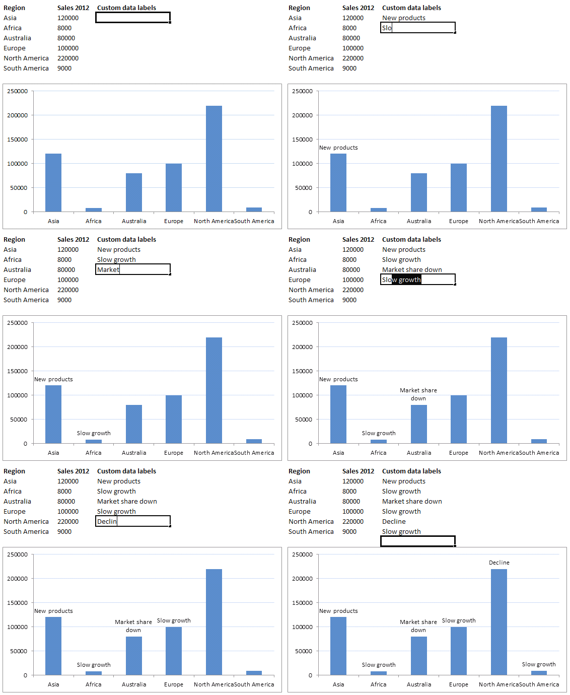
Custom data labels in a chart | Get Digital Help - Microsoft Excel resource
SAS Tutorials: User-Defined Formats (Value Labels) - Kent State University Typically, you will assign a unique value label to each unique data value, but it's also possible to assign the same label to a range of data values. Creating labels for each data value. The most common way of labeling data is to simply assign each unique code its own label. Here, the format LIKERT_SEVEN assigns distinct labels to the values 1 ...

How to create Custom Data Labels in Excel Charts – Efficiency 365
DataLabel object (Excel) | Microsoft Docs Use DataLabels ( index ), where index is the data-label index number, to return a single DataLabel object. The following example sets the number format for the fifth data label in series one in embedded chart one on worksheet one. VB Copy Worksheets (1).ChartObjects (1).Chart _ .SeriesCollection (1).DataLabels (5).NumberFormat = "0.000"
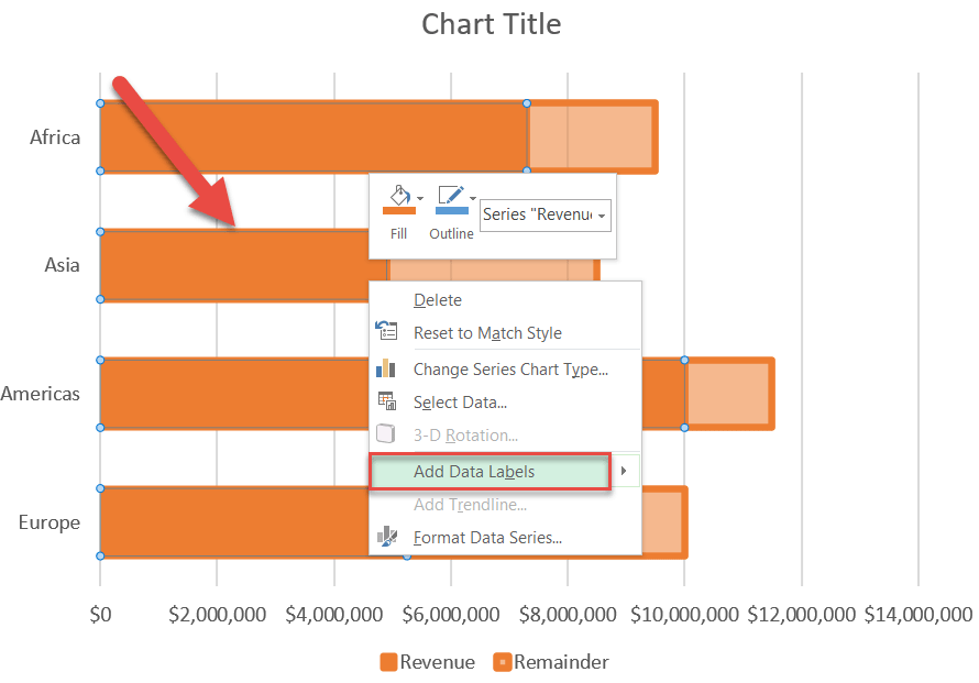
How to Create Progress Charts (Bar and Circle) in Excel - Automate Excel
Pivot Chart Data Label Formatting Question Hi, I have a pivot chart. I format the data labels, for example make the text larger or turn it. Every time I refresh the data the data label formatting reverts to the default. I have gone to the Pivot Chart options and made sure the Preserve cell formatting option is checked. How to I get around...
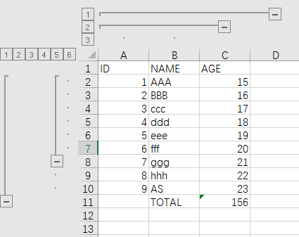
Labeling Excel data groups - Microsoft Community
DataLabels.ShowValue property (Excel) | Microsoft Docs This example enables the value to be shown for the data labels of the first series, on the first chart. This example assumes that a chart exists on the active worksheet. VB Copy Sub UseValue () ActiveSheet.ChartObjects (1).Activate ActiveChart.SeriesCollection (1) _ .DataLabels.ShowValue = True End Sub Support and feedback
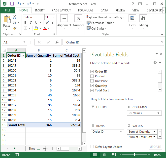
MS Excel 2013: Display the fields in the Values Section in a single column in a pivot table
How to Display Percentage in an Excel Graph (3 Methods) Then go to the More Options via the right arrow beside the Data Labels. Select Chart on the Format Data Labels dialog box. Uncheck the Value option. Check the Value From Cells option. Then you have to select cell ranges to extract percentage values. For this purpose, create a column called Percentage using the following formula: =E5/C5
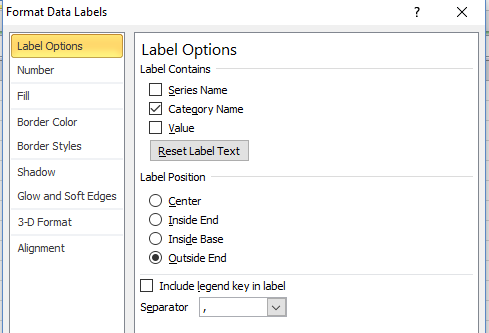
Create Dynamic Excel Chart Conditional Labels and Callouts
How to Use Excel Pivot Table Label Filters - Contextures Excel Tips Right-click a cell in the pivot table, and click PivotTable Options. In the PivotTable Options dialog box, click the Totals & Filters tab. In the Filters section, add a check mark to 'Allow multiple filters per field.'. Click the OK button, to apply the setting and close the dialog box.
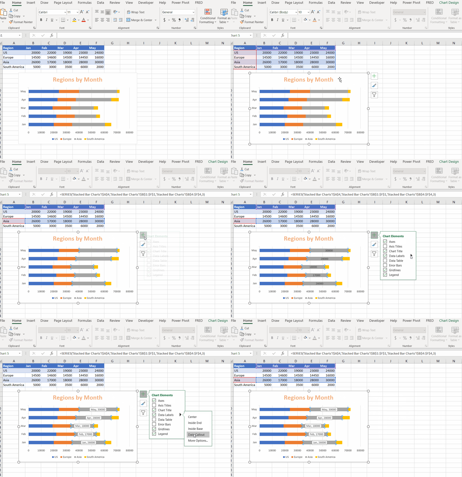
Excel Bar Charts - Clustered, Stacked - Template - Automate Excel
How to Find, Highlight, and Label a Data Point in Excel Scatter Plot ... By default, the data labels are the y-coordinates. Step 3: Right-click on any of the data labels. A drop-down appears. Click on the Format Data Labels… option. Step 4: Format Data Labels dialogue box appears. Under the Label Options, check the box Value from Cells . Step 5: Data Label Range dialogue-box appears.
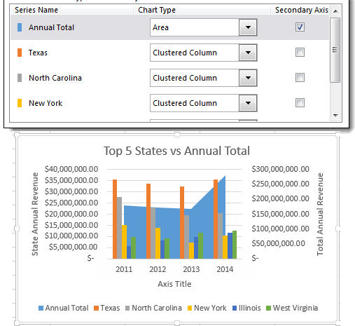
Working with Multiple Data Series in Excel | Pryor Learning Solutions
How to Add Total Values to Stacked Bar Chart in Excel Step 4: Add Total Values. Next, right click on the yellow line and click Add Data Labels. Next, double click on any of the labels. In the new panel that appears, check the button next to Above for the Label Position: Next, double click on the yellow line in the chart. In the new panel that appears, check the button next to No line:

Add label to Excel chart line • AuditExcel.co.za
Guide: How to Name Column in Excel | Indeed.com Select "Define Name" under the Defined Names group in the Ribbon to open the New Name window. Enter your new column name in the text box. Click the "Scope" drop-down menu and then "Workbook" to apply the change to all the sheets. 5. Clean all column names.
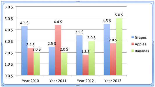
Format Number Options for Chart Data Labels in Excel 2011 for Mac
How do I make my Data Labels in my Excel chart have a square next to it ... I have a Pie chart and since there are many data I want to show values and % in the Data Labels. Those two are quite simple but I want to add the square next to the data labels that is the same as the one that appears in the Legends so it is easier to know what you are looking for.

Adding rich data labels to charts in Excel 2013 | Microsoft 365 Blog
How to format axis labels individually in Excel - SpreadsheetWeb The semicolon marks that you passed the next section. If you end with a semicolon, Excel thinks that there won't be a number format for the last section. Mark a single value [Cyan] [=60];General Set different colors for number ranges Since you have three sections for the conditions, you can set up to three colors.
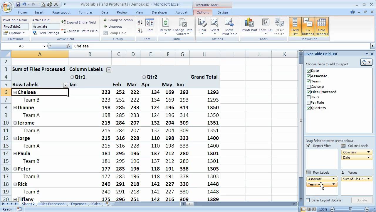
How to group row labels in Excel 2007 PivotTables (Excel 07-104) - YouTube
Custom Chart Data Labels In Excel With Formulas - How To Excel At Excel Follow the steps below to create the custom data labels. Select the chart label you want to change. In the formula-bar hit = (equals), select the cell reference containing your chart label's data. In this case, the first label is in cell E2. Finally, repeat for all your chart laebls.
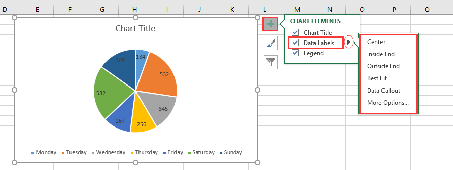
31 What Is Data Label In Excel - Labels Database 2020
VALUE Function - Formula, Examples, How to Use VALUE in Excel The VALUE Function [1] is categorized under Excel Text functions. It will convert a text string that represents a number into a number. Thus, the function will convert text that appears in a recognized format (a number, date, or time format) into a numeric value. In financial analysis, the VALUE function is not used much, as Excel automatically ...
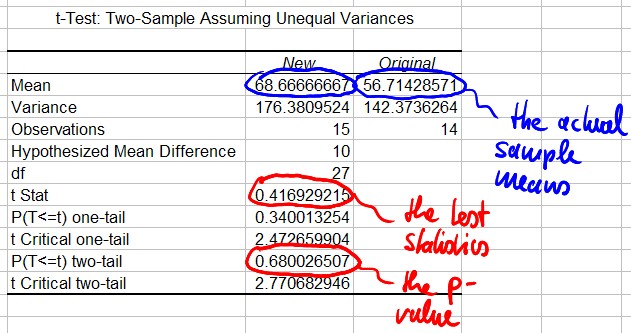
Testing for Difference of Means
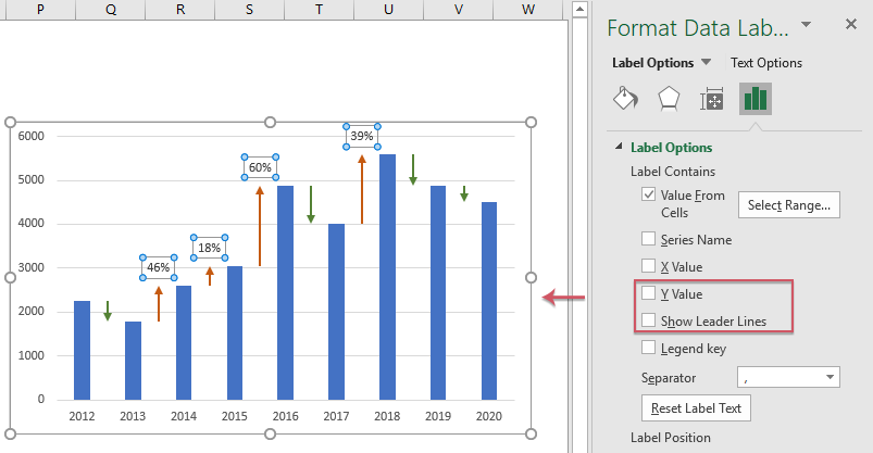
Create a column chart with percentage change in Excel
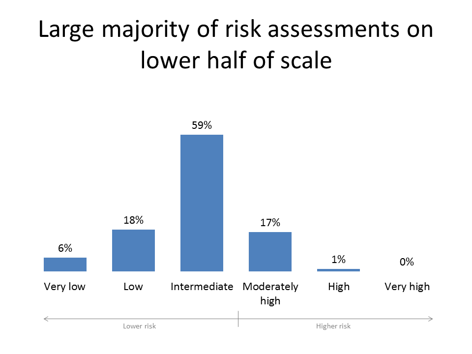
How to label graphs in Excel | Think Outside The Slide
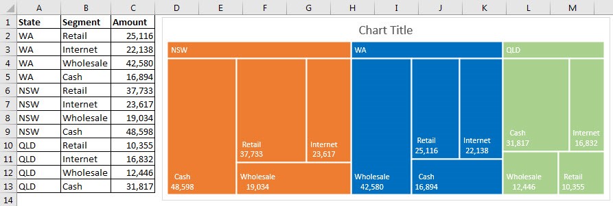
DFW Excel Experts Blog: Meet the Pie Chart's Brother, The TreeMap Chart
Post a Comment for "43 value data labels excel"